CMB Part 1: The “Smoking Gun” of the Big Bang
How the Cosmic Microwave Background — the Big Bang’s leftover radiation glow — continues to shed light on the birth of our Universe.
Image credit: ESA and the Planck Collaboration.
The announcement of the BICEP2 results, which showed the first evidence that gravitational waves may have been generated in our early Universe, also generated lots of interest in cosmology among scientists and non-scientists alike. The Cosmic Microwave Background (CMB), the so-called afterglow of the big bang, can become polarized in a particular fashion by gravitational waves, and it was this polarization signal which BICEP2 observed from its location at the south pole. But the Planck satellite has been the most recent experiment to weigh in, showing that a significant fraction of the BICEP2 result could have been due to not gravitational waves, but to nearby dust obscuring observations of the Cosmic Microwave Background itself.
We will need to wait for more data, both from a forthcoming collaboration between BICEP2 and Planck as well as from other experiments, to quantify just how much the dust may have masqueraded as a gravitational wave signal. One thing is for certain: science blogs and news sites will be keeping their attention focused on any new findings. This explainer is an attempt to help put those future articles about brand new research in the field of CMB cosmology into some context, starting with the basic science behind what the CMB is, how it was formed, and what it can tell us. The main focus here will be on the intensity of the CMB (which we call temperature), and in a future article I’ll talk more about polarization.
History
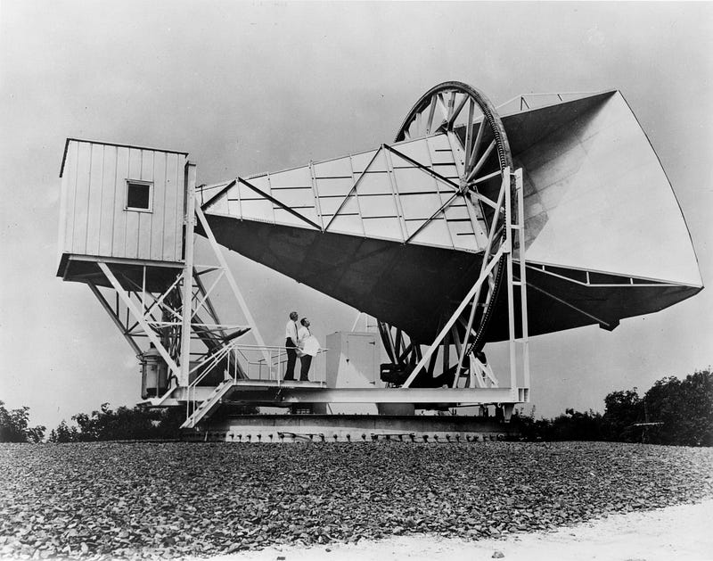
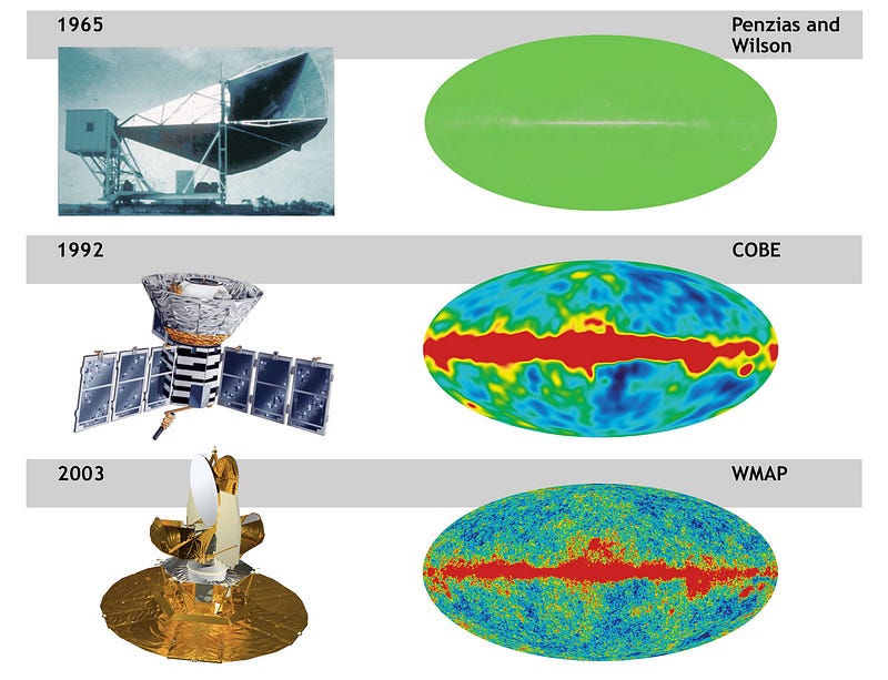
The first detection of the CMB in 1964 was an accident. Arno Penzias and Robert Wilson were working on an experiment at Bell Labs using balloon satellites as reflectors for transmitting microwave communications from one point on earth to another. To be able to do that, they needed to understand any possible noise that might contaminate their measurements. They had done an excellent job of accounting for all of them except one: the uniform 2.73 Kelvin (-450 degrees Fahrenheit) microwave radiation background which turned out to originate from 380,000 years after the big bang.
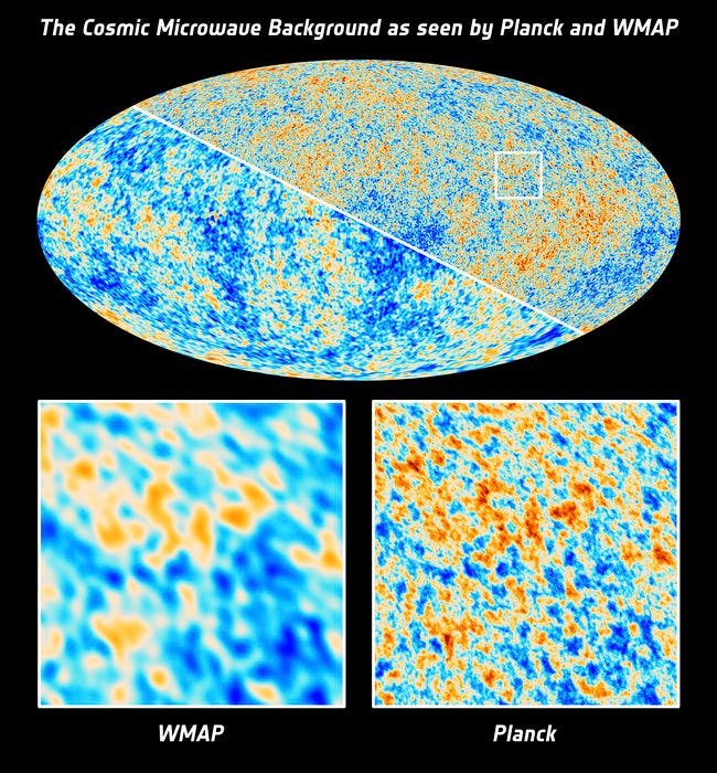
Since that initial detection by Arno Penzias and Robert Wilson (for which they won the Nobel Prize in Physics in 1978), several experiments here on Earth and out in space have measured the CMB with increasing precision. In 1992 the Cosmic Background Explorer (CoBE) showed the first observations of the CMB temperature anisotropies — tiny changes in temperature that are 100,000 times smaller than the uniform 2.73 Kelvin background average. The Wilkinson Microwave Anisotropy Probe (WMAP) expanded our full-sky knowledge of those temperature anisotropies in 2003, and in 2013 Planck gave us our most precise measurement to date. These continued improvements measured not only finer and finer temperature details, but also progressively smaller angular scales.
What is the CMB?
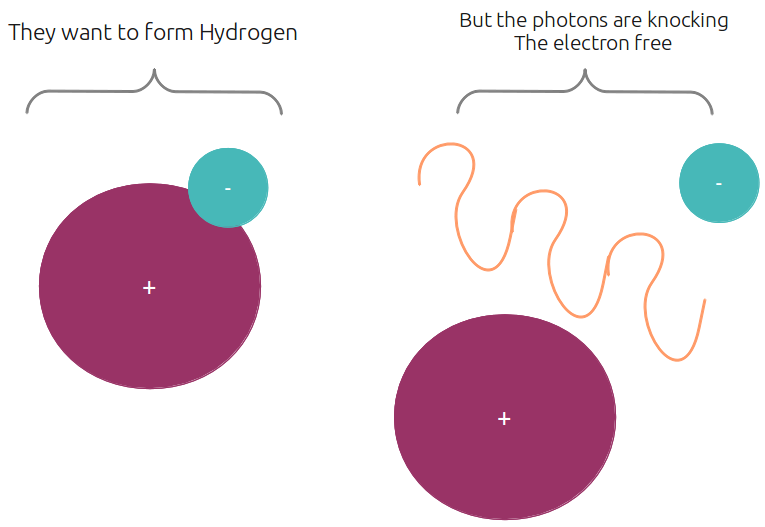
Before the CMB was formed, the ordinary components of the Universe were limited mostly to light (also called photons), hydrogen and helium nuclei, and free electrons. (Yes, there were also neutrinos and dark matter, but that’s a story for another time.) Since free electrons are negatively charged, they interact with photons through a process called Thomson scattering. If a photon and an electron cross paths, they will bounce off of one another just like two billiard balls. During this era the photons had a lot of energy, and the mean temperature of the Universe at this time was greater than 3000 Kelvin. The high temperature is exactly what kept the electrons free, since the photons had an energy greater than the atoms’ ionization energy: the amount of energy needed to knock an electron off of a nucleus. Instead of allowing them to stay bound to the positively charged hydrogen and helium nuclei to form neutral atoms, the energetic photons would kick an electron free the moment it combined with a nucleus.
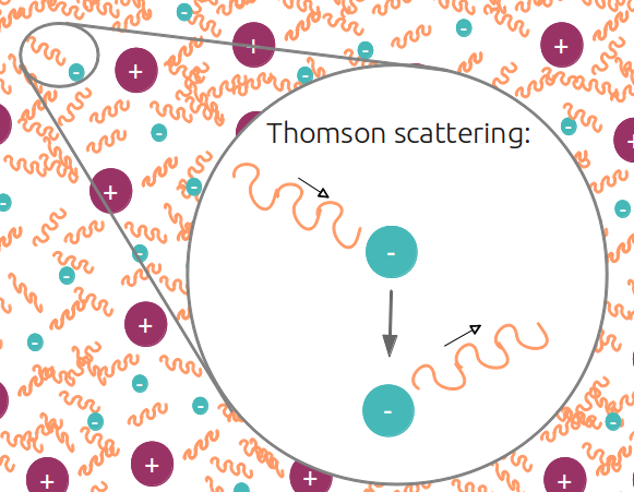
These two effects, photons making sure all nuclei remained ionized and photons interacting frequently with electrons, lead to important consequences. The high interaction rate means that a photon can’t travel far before it bounces off of an electron and changes direction. Think of driving in a thick fog, where the headlights of a car in front of you are obscured because the light from each bulb scatters off of the intervening water molecules. This is what is happening in the Universe before the formation of the CMB — nearby light is completely obscured by the fog of free electrons (often articles will refer to this period as the Universe being opaque). The combination of opaqueness and Thomson scattering is what gives the CMB its uniform 2.73K in all directions.
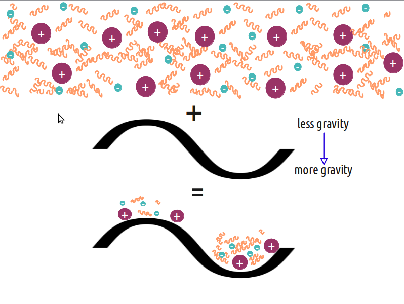
We also know that there should be tiny fluctuations around the uniform CMB temperature, since the high interaction rates mean that where the matter in the Universe goes, the photons will go too. You might often hear that the CMB can give us information about the dark matter content of the Universe, or that the hot and cold patterns in the CMB maps correspond to under- and over-dense areas, and this is why. Dark matter doesn’t interact regularly with ordinary matter, so it is able to clump into dense areas while the photons are still caught in the free-electron fog. The gravitational attraction of the clumps of dark matter pull the nuclei and electrons together, which bring the photons along with them.
So the temperature fluctuations of the photons that we observe in the CMB are direct tracers of where the matter was located more than 13 billion years ago. (If the fact that cosmologists have been able to observe the CMB isn’t impressive enough, the observed temperature fluctuations are 100,000 times smaller than the 2.73 Kelvin uniform background: on the scale of microKelvins!)
At the same time, space itself was expanding, causing the wavelength of the photons to be stretched along with it. The energy of a photon is related to its wavelength, so a longer wavelength means less energy. Eventually, the expansion of space stretches the photon wavelength enough that the photon energy drops below the ionization energy needed to keep electrons free. As soon as this happens, electrons combine with nuclei to produce neutral hydrogen and helium (among a few other things) and photons are suddenly able to stream outward, unimpeded.
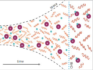
The point when neutral atoms form is known as recombination, and often this is described as the Universe becoming transparent. Since photons are now outside of the free-electron fog they can travel uninterrupted toward what will eventually become Earth and our CMB detectors! There is a brief moment between photons and electrons scattering off of one another (Universe being opaque) and neutral atoms forming (Universe becoming transparent) which is known as the surface of last scattering. This brief moment is exactly the picture the CMB is showing us. Because the Universe was opaque before the surface of last scattering, we literally cannot see anything before the time of the CMB using optical detectors.
But what about those plots?
The best way to get at the information contained in the maps of the CMB that we have is by computing its power spectrum, and you’re likely to have seen at least one in a popular article about the subject. The connection between the hot and cold spots we observe might seem like a stretch, but it’s actually pretty simple.
To understand what the connection is, we’ll first focus on a simple wave pattern. Any irregular smooth wave that you see or can draw has an important mathematical property: it can be written as a sum of many different, regular wave patterns with specific frequencies and different strengths. The wave itself is in real-space, meaning that we can plot it on an x and y axis. But we can also describe the exact same wave in harmonic-space, meaning we plot the frequencies needed in the sum to describe the original as a function of how strong each individual frequency must be. The gif below does an excellent job showing the connection between a wave pattern, how it can be broken into a sum of many different frequency, and how that relates to the harmonic-space plot. For people with a little more background math knowledge, this is simply a Fourier transform.
In addition to talking about a wave made from a single line, we can talk about a wave on a surface. This is exactly what the picture of the CMB is — a pattern of hot spots (peaks) and cold spots (troughs) imprinted on the surface of last scattering. Instead of showing one picture of the CMB temperature fluctuations, we can write it as a sum of many different patterns, each one corresponding to a specific mode or multipole.
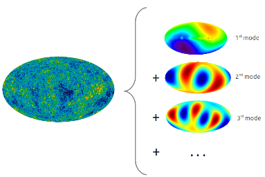
The CMB power spectrum plots you see tell you how strong each individual mode must be, so that when they’re summed together they reproduce the total CMB picture.
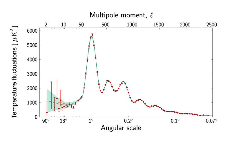
The brilliant thing about power spectra for cosmology is that we can make predictions for what it should look like based on properties we think the Universe has. The standard model for cosmology is called LambdaCDM, for Lambda (Dark Energy) Cold Dark Matter, and it fits the CMB temperature power spectrum remarkably well for most multipoles. The smallest multipoles (which correspond to large distance separations on the sky) seem to show some peculiarities, though, and many of those issues have been summarized very well here.
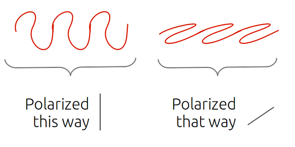
The discussion so far has been entirely about the temperature of the CMB observations, but the CMB photons also have polarization. Since light is an electromagnetic wave, it has an intensity and direction oriented with respect to a reference coordinate system. The direction the wave is oriented is its polarization, and the reason polarized sunglasses are so good at blocking glare. They preferentially filter out light waves that are oriented in the same direction, usually from being reflected off of a flat surface. The polarization of the CMB (which comes in two flavors, E-modes and B-modes) can be broken down into a power spectrum in the same way that the temperature fluctuations can be.
These additional power spectra add even more information about our early universe, including the possibility that they provide evidence for primordial gravitational waves. Do they really provide that evidence, though? That’s exactly the conflict between Planck and BICEP2 that scientists are attempting to untangle right now, with results forthcoming in just a few weeks!
This article was written by Amanda Yoho, a graduate student in theoretical and computational cosmology at Case Western Reserve University. You can reach her on Twitter at @mandaYoho. Come back in October for Part 2, where she’ll take us deeper into the science of the CMB!
Leave your comments at the Starts With A Bang forum on Scienceblogs!