The Big Theoretical Physics Problem At The Center Of The ‘Muon g-2’ Puzzle

The Big Theoretical Physics Problem At The Center Of The ‘Muon g-2’ Puzzle
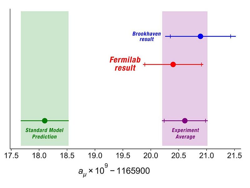
In early April, 2021, the experimental physics community announced an enormous victory: they had measured the muon’s magnetic moment to unprecedented precision. With the extraordinary precision achieved by the experimental Muon g-2 collaboration, they were able to measure the spin magnetic moment of the muon not only wasn’t 2, as originally predicted by Dirac, but was more precisely 2.00116592040. There’s an uncertainty in the final two digits of ±54, but not larger. Therefore, if the theoretical prediction differs by this measured amount by too much, there must be new physics at play: a tantalizing possibility that has justifiably excited a great many physicists.
The best theoretical prediction that we have, in fact, is more like 2.0011659182, which is significantly below the experimental measurement. Given that the experimental result strongly confirms a much earlier measurement of the same “g-2” quantity for the muon by the Brookhaven E821 experiment, there’s every reason to believe that the experimental result will hold up with better data and reduced errors. But the theoretical result is very much in doubt, for reasons everyone should appreciate. Let’s help everyone — physicists and non-physicists alike — understand why.
The Universe, as we know it, is fundamentally quantum in nature. Quantum, as we understand it, means that things can be broken down into fundamental components that obey probabilistic, rather than deterministic, rules. Deterministic is what happens for classical objects: macroscopic particles such as rocks. If you had two closely-spaced slits and threw a small rock at it, you could take one of two approaches, both of which would be valid.
- You could throw the rock at the slits, and if you knew the initial conditions of the rock well enough — its momentum and position, for example — you could compute exactly where it would land.
- Or, you could throw the rock at the slits, and simply measure where it lands a certain time later. Based on that, you could infer its trajectory at every point along its journey, including which slit it went through and what its initial conditions were.
But for quantum objects, you can’t do either of those. You could only compute a probability distribution for the various outcomes that could have occurred. You can either compute the probabilities of where things would land, or the probability of various trajectories having occurred. Any additional measurement you attempt to make, with the goal of gathering extra information, would alter the outcome of the experiment.
That’s the quantum weirdness we’re used to: quantum mechanics. Generalizing the laws of quantum mechanics to obey Einstein’s laws of special relativity led to Dirac’s original prediction for the muon’s spin magnetic moment: that there would be a quantum mechanical multiplicative factor applied to the classical prediction, g, and that g would exactly equal 2. But, as we all now know, g doesn’t exactly equal 2, but a value slightly higher than 2. In other words, when we measure the physical quantity “g-2,” we’re measuring the cumulative effects of everything that Dirac missed.
So, what did he miss?
He missed the fact that it’s not just the individual particles that make up the Universe that are quantum in nature, but also the fields that permeate the space between those particles must also be quantum. This enormous leap — from quantum mechanics to quantum field theory — enabled us to calculate deeper truths that aren’t illuminated by quantum mechanics at all.
The idea of quantum field theory is simple. Yes, you still have particles that are “charged” in some variety:
- particles with mass and/or energy having a “gravitational charge,”
- particles with positive or negative electric charges,
- particles that couple to the weak nuclear interaction and have a “weak charge,”
- or particles that make up atomic nuclei having a “color charge” under the strong nuclear force,
but they don’t just create fields around them based on things like their position and momentum like they did under either Newton’s/Einstein’s gravity or Maxwell’s electromagnetism.
If things like the position and momentum of each particle have an inherent quantum uncertainty associated with them, then what does that mean for the fields associated with them? It means we need a new way to think about fields: a quantum formulation. Although it took decades to get it right, a number of physicists independently figured out a successful method of performing the necessary calculations.
What many people expected to happen — although it doesn’t quite work this way — is that we’d be able to simply to fold all the necessary quantum uncertainties into the “charged” particles that generate these quantum fields, and that would allow us to compute the field behavior. But that misses a crucial contribution: the fact that these quantum fields exist, and in fact permeate all of space, even where there are no charged particles giving rise to the corresponding field.
Electromagnetic fields exist even in the absence of charged particles, for instance. You can imagine waves of all different wavelengths permeating all of space, even when no other particles are present. That’s fine from a theoretical perspective, but we’d want experimental proof that this description was correct. We already have it in a couple of forms.
- The Casimir Effect: you can put two conducting parallel plates close together in a vacuum, and measure an electric force due to the lack of certain wavelengths (since they’re forbidden by electromagnetic boundary conditions) in between the two plates.
- Vacuum birefringence: in regions with very strong magnetic fields, like around pulsars, intervening light becomes polarized as empty space itself must be magnetized.
In fact, the experimental effects of quantum fields have been felt since 1947, when the Lamb-Retherford experiment demonstrated their reality. The debate is no longer over whether:
- quantum fields exist; they do.
- the various gauges, interpretations, or pictures of quantum field theory are equivalent to one another; they are.
- or whether the techniques we use to calculate these effects, which were the subject of numerous mathematics and mathematical physics debates, are robust and valid; they are.
But what we do have to recognize is — as in the case with many mathematical equations that we know how to write down — that we cannot compute everything with the same straightforward, brute-force approach.
The way we perform these calculations in quantum electrodynamics (QED), for example, is we do what’s called a perturbative expansion. We imagine what it would be like for two particles to interact — like an electron and and electron, a muon and a photon, a quark and another quark, etc. — and then we imagine every possible quantum field interaction that could happen atop that basic interaction.
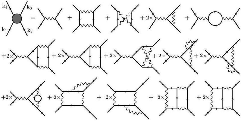
This is the idea of quantum field theory that’s normally encapsulated by their most commonly-seen tool to represent calculational steps that must be taken: Feynman diagrams, as above. In the theory of quantum electrodynamics — where charged particles interact via the exchange of photons, and those photons can then couple through any other charged particles — we perform these calculations by:
- starting with the tree-level diagram, which assumes only the external particles that interact and possesses no internal “loops” present,
- adding in all the possible “one-loop” diagrams, where one additional particle is exchanged, allowing for larger numbers of Feynman diagrams to be drawn,
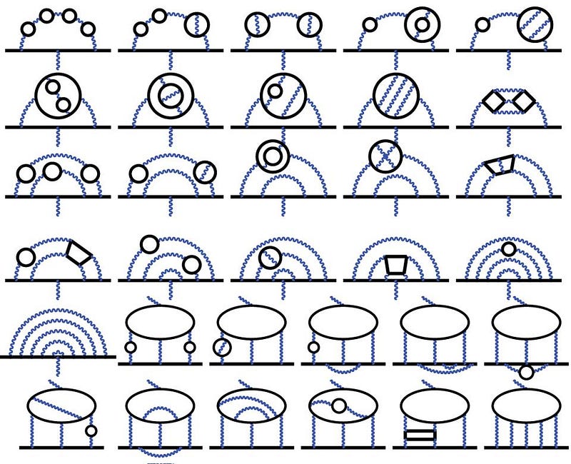
- then building on those to allow for all possible “two-loop” diagrams to be drawn, etc.
Quantum electrodynamics is one of the many field theories we can write down where this approach, as we go to progressively higher “loop orders” in our calculations, gets more and more accurate the more we calculate. The processes at play in the muon’s (or electron’s, or tau’s) spin magnetic moment have been calculated beyond five-loop order recently, and there’s very little uncertainty there.
The reason this strategy works so well is because electromagnetism has two important properties to it.
- The particle that carries the electromagnetic force, the photon, is massless, meaning that it has an infinite range to it.
- The strength of the electromagnetic coupling, which is given by the fine-structure constant, is small compared to 1.
The combination of these factors guarantees that we can calculate the strength of any electromagnetic interaction between any two particles in the Universe more and more accurately by adding more terms to our quantum field theory calculations: by going to higher and higher loop-orders.
Electromagnetism, of course, isn’t the only force that matters when it comes to Standard Model particles. There’s also the weak nuclear force, which is mediated by three force-carrying particles: the W-and-Z bosons. This is a very short-range force, but fortunately, the strength of the weak coupling is still small and the weak interactions are suppressed by large masses possessed by the W-and-Z bosons. Even though it’s a little more complicated, the same method — of expanding to higher-order loop diagrams — works for computing the weak interactions, too. (The Higgs is also similar.)
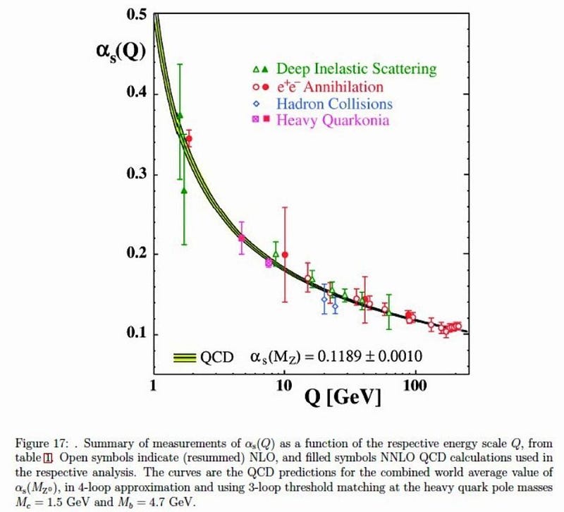
But the strong nuclear force is different. Unlike all of the other Standard Model interactions, the strong force gets weaker at short distances rather than stronger: it acts like a spring rather than like gravity. We call this property asymptotic freedom: where the attractive or repulsive force between charged particles approaches zero as they approach zero distance from one another. This, coupled with the large coupling strength of the strong interaction, makes this common “loop-order” method wildly inappropriate for the strong interaction. The more diagrams you calculate, the less accurate you get.
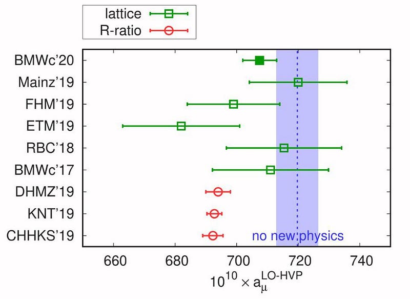
This doesn’t mean we have no recourse at all in making predictions for the strong interactions, but it means we have to take a different approach to our normal one. Either we can try to calculate the contributions of the particles and fields under the strong interaction non-perturbatively — such as via the methods of Lattice QCD (where QCD stands for quantum chromodynamics, or the quantum field theory governing the strong force) — or you can try and use the results from other experiments to estimate the strength of the strong interactions under a different scenario.
If what we were able to measure, from other experiments, was exactly the thing we don’t know in the Muon g-2 calculation, there would be no need for theoretical uncertainties; we could just measure the unknown directly. If we didn’t know a cross-section, a scattering amplitude, or a particular decay property, those are things that particle physics experiments are exquisite at determining. But for the needed strong force contributions to the spin magnetic moment of the muon, these are properties that are indirectly inferred from our measurements, not directly measured. There’s always a big danger that a systematic error is causing the mismatch between theory and observation from our current theoretical methods.
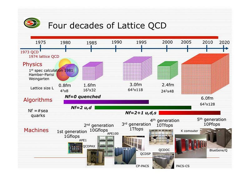
On the other hand, the Lattice QCD method is brilliant: it imagines space as a grid-like lattice in three dimensions. You put the two particles down on your lattice so that they’re separated by a certain distance, and then they use a set of computational techniques to add up the contribution from all the quantum fields and particles that we have. If we could make the lattice infinitely large, and the spacing between the points on the lattice infinitely small, we’d get the exact answer for the contributions of the strong force. Of course, we only have finite computational power, so the lattice spacing can’t go below a certain distance, and the size of the lattice doesn’t go beyond a certain range.
There comes a point where our lattice gets large enough and the spacing gets small enough, however, that we’ll get the right answer. Certain calculations have already yielded to Lattice QCD that haven’t yielded to other methods, such as the calculations of the masses of the light mesons and baryons, including the proton and neutron. After many attempts at predicting what the strong force’s contributions to the g-2 measurement of the muon ought to be over the past few years, the uncertainties are finally dropping to become competitive with the experimental ones. If the latest group to perform that calculation has finally gotten it right, there is no longer a tension with the experimental results.
Assuming that the experimental results from the Muon g-2 collaboration hold up — and there’s every reason to believe they will, including the solid agreement with the earlier Brookhaven results — all eyes will turn towards the theorists. We have two different ways of calculating the expected value of the muon’s spin magnetic moment, where one agrees with the experimental values (within the errors) and the other does not.
Will the Lattice QCD groups all converge on the same answer, and demonstrate that not only do they know what they’re doing, but that there’s no anomaly after all? Or will Lattice QCD methods reveal a disagreement with the experimental values, the same way that they presently disagree with the other theoretical method we have that presently disagrees so significantly with the experimental values we have: of using experimental inputs instead of theoretical calculations?
It’s far too early to say, but until we have a resolution to this important theoretical issue, we won’t know what it is that’s broken: the Standard Model, or the way we’re presently calculating the same quantities we’re measuring to unparalleled precisions.
Starts With A Bang is written by Ethan Siegel, Ph.D., author of Beyond The Galaxy, and Treknology: The Science of Star Trek from Tricorders to Warp Drive.